Basic Steps to Analyzing Data
TRIOS contains a variety of analysis functions specific to the selected data. To access these functions, follow these general instructions:
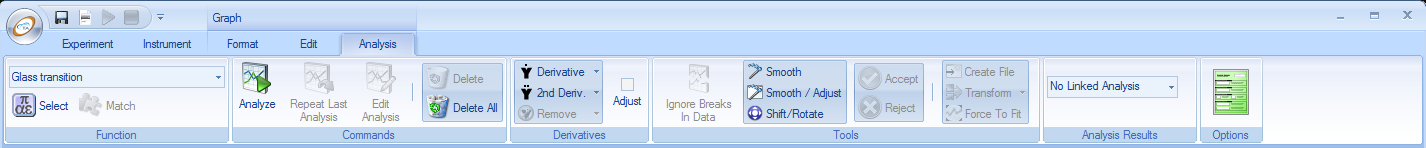
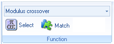
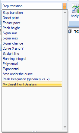
- From the Function toolbar, select the desired analysis/model using either of the following methods:
- Click the arrow of the upper drop-down list and select your desired analysis/model.
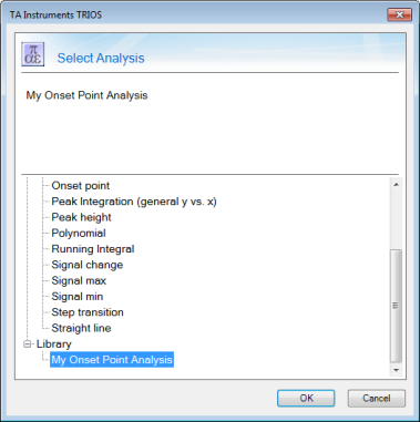
- Click Select
 , select the desired analysis/model from the dialogue box, and click OK. A brief description of each option displays.
- Click Analyze.
- Once you have performed an analysis, the Edit Analysis button (on the Commands toolbar of the Analysis tab) becomes available. Click Edit Analysis to verify and/or adjust the associated function settings. Refer to Editing Analysis for more information.
- If the parameters selected in the graph do not match the parameters used in the function, the Match icon on the Function toolbar is active. Click Match to load the model parameters into the graph. If you do not match the parameters, the Start button is grayed out and the analysis cannot be performed.
- If a subset of the selected curve is to be analyzed, select the Cursors tab to display the appropriate analysis cursors. Use them to specify the desired range of data to be analyzed. To position the analysis cursors, use one of the following methods:
- Click on the markers using the mouse and drag them to your desired locations.
- Double-click on the desired locations on the cursor to move the markers. The cursor will move to that selected location in the order performed.
- Open the analysis settings using the Edit Analysis button and enter the desired analysis limits on the Cursorstab.
- Alternatively, select the analysis region by dragging the mouse of the desired region, then immediately click Start.
- Click Start to begin the analysis (or Cancel to exit the analysis function).
- At the end of the computation (see Running Models), the analysis/model curve is displayed on the graph with its associated legend. You can view the complete results within the analysis Settings window.
- Click Create File (if available for the selected model) to create a separate data file of the analysis results, where applicable.
- NOTE: This function is only available for the continuous and discrete relaxation and retardation spectra.
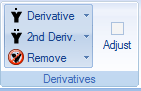
The Derivatives Toolbar
To add a derivative curve to the graph, follow the instructions below:
- Several derivative and smoothing techniques are available in TRIOS. The desired options are set within the TRIOS Options > Analysis page. Verify the desired technique is selected.
- To use the Derivatives toolbar, click a point on the curve used to calculate the derivative signal.
- From the Graph > Analysis tab > Derivatives toolbar, select between the following options:
- Click Derivative to display first derivative for the selected curve (variable) using the default smoothing value shown. Select between the following options:
- Wrt (with regard to) X: The derivative is calculated versus the current x axis variable.
- Wrt Time: The derivative is calculated versus the associated time variable.
- Wrt Temperature: The derivative is calculated versus the associated temperature variable.
- Click 2nd Deriv. to display second derivative for the selected curve (variable) using the default smoothing value shown. Select between the following options:
- Wrt X: The derivative is calculated versus the current x axis variable.
- Wrt Time: The derivative is calculated versus the associated time variable.
- Wrt Temperature: The derivative is calculated versus the associated temperature variable.
- NOTE: If you wish to change or adjust the derivative smoothing interval interactively, click the Adjust option before making the selection above. The Derivative Adjust window appears, which allows you to adjust the smoothing to a desired level by either 1) moving the slider bar, or 2) entering a value while simultaneously viewing the smoothed signal and comparing it to the original data. When satisfied, click OK.
- Click Remove to remove the derivatives. Select between the following options:
- This removes the selected derivative.
- All removes all derivatives.
See also
Derivatives
Setting TRIOS Options
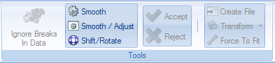
Using Analysis Tools
For information regarding using the Analysis tools (toolbar shown below), refer to the Using Analysis Tools Help topic.
Back to top
Deleting an Analysis
If you wish to delete the analysis once it is performed:
- Select the annotation box in the graph.
- Select Analysis tab > Commands toolbar > Delete Alternatively, right-click in the annotation and select Delete from the pop-up menu. This function removes all lines and labels associated with the analysis.
- If you wish to delete all analyses, click Delete All from the Commands toolbar.
Editing an Analysis
If you wish to alter an analysis annotation, double-click inside the annotation box and alter the text as needed. Refer to Adding Objects to a Graph.
To edit an analysis:
- Click Edit Analysis on the ribbon, or right-click a point on the graph and select Edit analysis.
- A dialog box displays, allowing you to edit the cursors, parameters, appearance, and labels for that analysis. For models that produce a fit line, additional editable options include results and point values. Click the appropriate tab and make the needed changes.
- Cursors: If applicable, display the limits which will be used for analysis and allow manual entry.
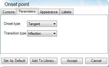
- Parameters:
Defines the input parameters and settings corresponding to the selected function. Settings can only be changed prior to selecting Start.
- Appearance:
Use to customize the color and shading options corresponding to the selected completed analysis.
- Labels
:
Use to specify the information (label) shown on the graph corresponding to the selected completed analysis.
- Results:
Provides a complete summary of the parameters and results associated with the selected completed analysis.
- Point Values: Allows one or more theoretical points to be calculated from a specified x value based on the completed analysis.
The information displayed in these options varies based on the selected analysis/model.
- Make one of the following selections to complete your changes:
- Accept to accept your changes.
- Cancel to delete the analysis (if auto-edit is selected in the ribbon and it is the first time you have created the model) or revert your changes to how the model appeared upon entering edit mode.
- Set As Default to use your settings as the default settings.
- Add to Libraryto save the parameters of a particular analysis to be used for another analysis of that type. Refer to Analysis Library for more information.
Cursors
The Cursors tab allows manual entry of the analysis limits. The number of fields vary based on the selected functions and its input settings.

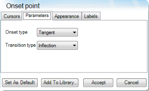
Parameters
The Parameters settings allows configuration of the parameters for an analysis. Depending on the function chosen the information in this window will vary.
Appearance
The Appearance tab allows you to further customize the result label (if applicable).
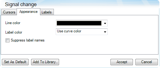
- Line color: Manual color selection, automatic color from bank, or use curve color
- Label color: Manual color selection, automatic color from bank, or use curve color
- Label names: Select the checkbox to suppress label names, for example 1.2345. Deselect to display label names, for example Max y: 1.2345 .
If you wish to save your selections, click Set as Default.
Back to top
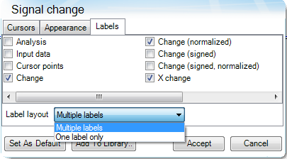
Labels
The Labels tab allows you to specify the information (label) shown on the graph corresponding to the selected completed analysis. Check those labels you wish to display.
If you wish to save your selections, click Set as Default.
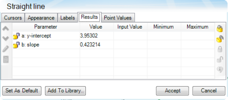
Results
The Results window shows the parameters that will be fitted for the currently-selected model. It also displays details of the analysis, such as the Parameter Values of the parameter fitted during the analysis, the Input Values, and the Minimum and Maximum values.
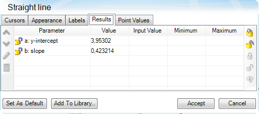
To the left of the parameter name is an icon showing the input status for that parameter. The input status is indicated by an lock icon in one of the following states:
-
 Unlocked – the analytical routine has freedom over fitting of the parameter, including estimation of the initial guess.
-
 Unlocked with hint – the analytical routine has freedom over fitting of the parameter but with a user-entered initial guess.
-
 Locked – the parameter takes the value entered by the user and is not fitted.
To set the status for a parameter:
- Click the cell of the parameter name.
- Select one of the following options from the toolbar icons:
- Locked

- Unlocked

- Provide a starting estimate

- Edit

- Unlock all
 or Lock all
  sets the input status for all parameters for the model
For a parameter that is locked or unlocked with hint, it is then necessary to specify the parameter value or parameter initial guess, respectively. To do so, click in the Value column for the parameter and enter the desired value.
For any parameter that is unlocked, either with or without a hint, it is possible to specify the minimum and / or maximum value that the parameter may take. The analytical routine will not exceed the specified limit(s) when estimating the parameter. To set a limit, click in the Minimum or Maximum column for the parameter and enter the desired value.
If you wish to save your selections, click Set as Default.
Point Values
Point values can be calculated using the analysis parameters by clicking the Point Values tab. Calculated values are automatically added to the analysis label on the graph. Note: Point values are only available for models that produce a fit line.
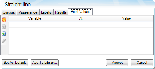
To manage point values:
- Select Add
 to add a new point to the point value window.
- Select Edit
 to edit the default value.
- Once set up, the same point values are used by every analysis. Remove point values using the Delete
 / Delete All
 .
.
Back to top
Analysis Library
The Analysis Library allows you to save your analysis parameters, storing your settings in the Function toolbar of the ribbon so that you can easily select and apply your saved analysis parameters to your graph.
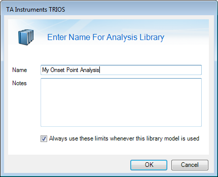
Adding an Analysis to the Analysis Library
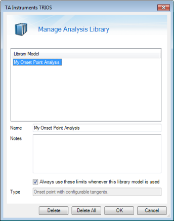
When you either select Add to Library from the dialog box while editing an analysis (see above) or right-click a point on the graph and select Add to Analysis Library, you are prompted to name the model, as shown below. Add identifying information to the Notes section, if desired. Select Always use these limits whenever this library model is used to also save the cursor points. Click OK to save your changes or Cancel to dismiss them.
Applying your saved analysis
When you add a saved analysis to the Analysis Library, it will appear in the list of analyses. To apply your saved analysis, select it from the drop-down menu on the Function toolbar, or click Select and choose it from the dialog box.
Managing the Analysis Library
To rename or delete an analysis saved in the Analysis Library, right-click a point in the graph and select Manage Analysis Library. Your created analyses appear in the Library Model list.
To rename the analysis, select it from the list and edit the text in the Name field and click OK.
To delete a single analysis, click Delete. To delete all analyses in the list, click Delete All.
Click OK when finished to return to the graph, or Cancel to dismiss your changes.
Available Analysis Options
See Analysis Models for the list of available analysis options.